Building virtual forest landscapes to support forest management: the challenge of parameterization

Marco Mina,^a,* Sebastian Marzini,^a,b  Alice Crespi, ^c Katharina Albrich. ^d,e

a: Eurac Research, Institute for Alpine Environment, Bolzano, Italy.
b: Free University of Bolzano, Faculty of Agricultural, Environmental and Food Sciences, Italy.
c: Eurac Research, Center for Climate Change and Transformation, Bolzano, Italy.
d: Natural Resources Institute Finland (LUKE), Helsinki, Finland.
e: University of Eastern Finland, School of Forest Sciences, Joensuu, Finland
*Corresponding author: E-mail: [email protected]

Citation: Mina M, Marzini S, Crespi A, Albrich K. 2025. Building virtual forest landscapes to support forest management: the challenge of parameterization. For. Monit. 2(1): 49-96. https://doi.org/10.62320/fm.v2i1.19

Received:  15 January 2024 / Accepted:  16 February 2025 / Published: 28 February 2025

Copyright: © 2025 by the authors

---

ABSTRACT

Simulation models are important tools to study the impacts of climate change and natural disturbances on forest ecosystems. Being able to track tree demographic processes in a spatially explicit manner, process-based forest landscape models are considered the most suitable to provide robust projections that can aid decision-making in forest management. However, landscape models are challenging to parameterize and setting up new study areas for application studies largely depends on data availability. The aim of this study is to demonstrate the parameterization process, including model testing and evaluation, for setting up a study area in the Italian Alps in a process-based forest landscape model using available data. We processed soil, climate, carbon pools, vegetation, disturbances and forest management data, and ran iterative spin-up simulations to generate a virtual landscape best resembling current conditions. Our results demonstrated the feasibility of initializing forest landscape models with data that are typically available from forest management plans and national forest inventories, as well as openly available mapping products. Evaluation tests proved the ability of the model to capture the environmental constraints driving regeneration dynamics and inter-specific competition in forests of the Italian Alps, as well as to simulate natural disturbances and carbon dynamics. The model can subsequently be applied to investigate forest landscape development under a suite of future scenarios and provide recommendations for adapting forest management decisions.

Keywords: calibration, disturbance modelling, European Alps, forest landscape models, forest modelling, model initialization 

---

INTRODUCTION

Forests are vital components of Alpine landscapes and provide a wide range of ecosystem services to human society, such as habitat for biodiversity, timber, protection against natural hazards, and recreation (Gret-Regamey et al. 2012, Mina et al. 2017). Forests are crucial contributors to the global climate system and are often found at the center of discussions on climate change mitigation and nature-based adaptation solutions (Bonan 2008, Kaarakka et al. 2021). However, forests' capacity to maintain the provision of these important services is threatened by the impact of climate change and related natural disturbances (Millar and Stephenson 2015, Seidl et al. 2017, McDowell et al. 2020). Disturbances such as large windthrow events, insect outbreaks, and forest fires have significantly increased in Europe since the 1950s due to warming climate and other abiotic factors such as forest management (Patacca et al. 2023). Recent studies have shown that these disturbance events will likely be amplified by climate change (Seidl et al. 2017, Forzieri et al. 2021, Grünig et al. 2023). Given the recent increasing trend in tree mortality worldwide (ITMN 2025), new adaptations in forest management are needed to guarantee the future provision of key services provided by forests (Mina et al. 2017, Tognetti et al. 2022, Blattert et al. 2024). The ongoing debate regarding the role of forests in climate change mitigation calls for reliable tools that are able to assess how forests are likely to evolve in the coming decades (Verkerk et al. 2020, Pan et al. 2024).

In complement to empirical approaches, state-of-the-art modelling tools are needed to evaluate the long-term impact of environmental changes and potential forest adaptations in the future (Seidl 2017, Bugmann and Seidl 2022). Forest simulation models have become pivotal tools in forest resilience research (Shifley et al. 2017, Albrich et al. 2020b) and, in recent years, have been widely applied for supporting forest management in a changing environment (Fontes et al. 2010, Bosela et al. 2022). In particular, process-based forest landscape models, which can track tree demographic processes influencing forest dynamics in a spatially explicit manner, are considered the most suitable tools for investigating forest development under global change (Gustafson 2013, Bosela et al. 2022). These models account for species sensitivity to changing environmental conditions and can assess the potential impact of natural disturbances such as windthrow, insect outbreaks, and forest fires, which are drivers that cannot be disregarded anymore when studying forest ecosystem dynamics (Seidl et al. 2011). Such models are also powerful tools to quantify carbon stocks as they can track the development of carbon pools dynamically (Albrich et al. 2023). Additionally, being able to simulate the effect of management interventions, such models can be applied to assess the potential of different silvicultural strategies to boost forest resilience to global change (Rammer and Seidl 2015, Mina et al. 2022). Therefore, forest landscape models can provide key information to decision makers to assess the effect of long-term strategies in forest management and climate-smart forestry (Bosela et al. 2022, Holland et al. 2022).  

Despite their potential, the main challenge for applying such models lies in their parameterization (Scheller 2018, Reese et al. 2025). With the generic term parameterization, we herewith refer not only to the procedure of estimating parameters for ecological processes and statistical relationships within a model, but to the entire process required for setting up a new study area or a landscape for an application, which includes: model initialization (i.e., landscape and forest extent, biophysical and climate conditions, initial vegetation via spin-up simulations, information disturbances and/or management), model testing and calibration (at site- or landscape-level using e.g., inventory data), and final evaluation and/or validation. Compared to performing a simulation experiment, parameterizing an entirely new study area in forest landscape models can take a significant amount of time and effort, which – if executed in parallel with collecting and preparing all the necessary data – can easily take longer than a year of full-time work (Hof et al. 2024). Despite involving multiple methodological steps, which differ depending on the available data and on the complexity of the model, such parameterization process is usually condensed to short methodological sections or relegated to the supplementary material in articles describing model applications (Seidl et al. 2019, Mina et al. 2021, Thom et al. 2022). Only a few studies focused on parameterization and calibration processes for forest landscape models (Suárez-Muñoz et al. 2021, Willis et al. 2023). This is a gap in the existing literature. Although such studies may not present future projections of forest development, they are yet invaluable to other researchers as they offer practical examples of how to accurately establish a virtual forest landscape using existing environmental and forest management data. This type of methodological studies can help in speeding up successive calibration and initialization procedures required to apply forest landscape models in new regions. Successional processes and long-term projections in forest models are highly sensitive to initial conditions and model parameters, therefore manuscripts documenting the parameterization process for setting up new study areas for specific models should be promoted to foster further applications and reproducibility (Furniss et al. 2022).

The aim of this study is to demonstrate the process for setting up new study areas for the process-based forest landscape and disturbance model iLand (Rammer et al. 2024). Our goal is to provide detailed documentation on how to generate a virtual forest landscape that best resembles current vegetation conditions using data that are typically available for Italian forests. The documented process includes performing spin-up simulations with historic forest management regimes, which is needed to integrate all the legacies of past management and land use. The final goal of this parameterization process is a virtual replica of the forest in a study area that is ready for simulating forest dynamics and its evolution under future scenarios, including different forest management strategies. We also discuss the potential and challenges of using complex simulation models in the context of climate change adaptations.

MATERIALS AND METHODS

Study area

Our study area is located in the province of South Tyrol, in northern Italy (46°30’0”N, 11°21’0”E). It includes the upper portion of an inner alpine valley called Vinschgau in German or Val Venosta in Italian (hereafter Venosta). The region encompasses not merely a single valley, as is commonly implied when discussing landscape scales in mountainous areas, but rather constitutes a complex mountainous territory. In addition to the main Venosta valley, it incorporates three lateral valleys with various elevational gradients and expositions: the Val Mazia/Matschertal in the north, Val Trafoi/Trafoital in the southwest, and the Val di Solda/Suldental in the southeast (Figure 1). The latter two are both embedded within the Stelvio/Stilfs National Park. We selected this study area together with the regional forest services because it is representative of the multiplicity of forest types across the South Tyrol province (Autonomous Province of Bolzano/Bozen 2010). The study area was also designed to run future model applications separately on different, smaller landscapes. The elevation ranges from 850 meters (m) at the valley bottom to circa 2600 m above sea level (a.s.l). The extent of the overall area (hereafter project area) is 30,426 hectares (ha), of which 12,589 ha is covered by forest (hereafter stockable area). The layer of forest cover was obtained from the Copernicus high-resolution layers of forest-type product for the reference year 2018 at 10 m resolution (EEA 2018). Cells overlapping with agricultural and urban areas, as well as riparian forests and tree patches at the valley bottom close to urban settlements, were manually removed by orthophoto interpretation. This resulted in a clean delineation between forest and non-forest below approximately 900-1000 m a.s.l. (Figure 1). The uppermost border of the project area was delineated with the contour line at 2600 m a.s.l. We also left a buffer of approximately one kilometer in the direction east and west between the forest cover and the project area for light influence and for the seed belt (see further below).

Figure 1. The study area in the upper Venosta/Vinschgau and its three side landscapes (a- Val Mazia; b- Val Trafoi; c- Val Solda). The project area (i.e., boundaries of the biophysical and climate parameters) is highlighted with brighter colors, while the stockable forest area is shown with the black lines. Location of the study area within South Tyrol (red line) is shown in the small inset map. Photos show three different forests within the area: 1- a subalpine larch-Stone pine in Val Mazia; 2- a black pine-pubescent oak at the valley bottom; 3- a spruce forest under the Ortler mountain in Trafoi.

Simulation model

The focal model of this study is iLand, a process-based model that simulates demographic processes of trees, such as growth, dispersion, regeneration, and mortality, in a spatially explicit manner (Seidl et al. 2012a). The model can be applied with a multi-scale approach from the single tree to the stand to the landscape scale, giving the users ample flexibility in application (Rammer et al. 2024). Rather than modelling forest growth with empirical functions fit to measured data, the model simulates ecological mechanisms such as photosynthesis and carbon allocation explicitly. Primary productivity is directly influenced by climatic conditions (e.g., temperature, precipitation, solar radiation), CO₂ concentrations, soil nutrients, and competition for light (Thom et al. 2024). Regeneration accounts for seed availability and dispersal, and for seedling and sapling establishment (Holzer et al. 2024), while tree mortality is modelled probabilistically depending on tree age and external stress factors. In addition to being process-based – and thus suitable to make inferences under novel environmental conditions – iLand is capable of simulating forest disturbances (e.g., bark beetles, wind, fire) interactively with climate change (Dollinger et al. 2024). For instance, the wind disturbance module allows the simulation of a process-oriented manner the impact of a storm event on trees within the landscape, which depends on wind data and forest structure and composition (Seidl et al. 2014). Wind damages interact with simulated soil conditions (e.g., differentiating between tree uprooting and stem breakages depending on soil freezing) and are performed for all landscape cells with vertical differences over 10 meters, referred to as edges (Seidl et al. 2014). The bark beetle module emulates outbreaks of Ips typographus explicitly considering the beetle´s phenology, colonization, dispersal, and tree defense, as well as temperature-related overwintering (Seidl and Rammer 2017). A flexible management module also allows simulating forest management activities and silvicultural practices in relation to stand characteristics and changing environmental conditions (Rammer and Seidl 2015). Differently from other forest landscape models that estimate belowground biomass with allometric equations, iLand explicitly tracks above- and below-ground carbon pools and fluxes such as coarse woody debris, snags, stumps, soil organic matter, and can therefore be applied to study forest carbon dynamics (Albrich et al. 2023). To account for stochasticity in the simulations, the model is typically run for 10-20 replicates per scenario (Seidl et al. 2014, Dollinger et al. 2024). The model has already been calibrated for the main European forest species and has been widely applied across different landscapes in the Alps (Seidl et al. 2012b, Thom et al. 2018). Given its ability to project forest landscape dynamics under climate change and disturbance factors, the model can be applied to provide important recommendations to forest managers, pending that it is first initialized and calibrated in a study area that is of high interest to decision-makers.

Model initialization

The main inputs required by the model to be able to simulate forest dynamics are: 1) biophysical properties, 2) climate data, and 3) initial vegetation conditions. The first two are defined in an environment grid at a resolution of 100 m (cells referred to as resource units), while the third needs to be delineated at a horizontal resolution of 10 m (Rammer et al. 2024). Biophysical properties such as soil depth, texture, and plant-available nitrogen are considered to be homogenous at the level of resource unit and typically do not change during a simulation interval (Seidl et al. 2012a). Climate variables such as minimum and maximum temperature, precipitation, global radiation, and vapor pressure deficit are implemented as daily time series at the level of resource unit but are typically aggregated spatially into climate clusters – i.e., regions of the landscape with similar climatic conditions – to reduce the amount of data processed by the model (details in the section on Climate). Initial vegetation conditions consist of species- and size-specific data on live individual trees and regeneration. This is typically derived by combining available plot-level data (e.g., forest inventory) with spatially explicit products such as maps of forest management plans, canopy height from LiDAR, or maps of forest typologies describing current forest structure and composition. As this data is rarely available at high resolution for large areas, approximate forest conditions are often generated using spin-up simulations (see section on Vegetation). In this section, we describe the process of preparing all the necessary data for initializing the Venosta study area within iLand.

Biophysical parameters

Biophysical properties are important drivers of ecological processes (e.g., establishment, growth) acting in forest ecosystems at different spatial scale (Ehrenfeld et al. 2005). In iLand, hydrological balance and available soil water for plants are affected by soil properties such as soil depth and texture, while soil nitrogen has a direct effect on plant growth as a proxy for site fertility (Seidl et al. 2012a). For the Venosta study area, we made the best use of available data to derive high-resolution, spatially explicit datasets of soil properties and plant available nitrogen estimates. Additionally, as our aim was to set up the model with the dynamic carbon cycling module, we estimated current carbon pools by imputing data from forest inventory plots into forest-type maps within our study area (see below).

Soil depth and texture

We obtained soil depth and texture variables from soil maps that were developed for the administrative unit Vinschgau/Val Venosta in South Tyrol for a past research project (Interreg CH-IT IRKIS;  Zischg 2012). In that context, soil maps were derived by merging data from multiple sources such as forest-type map, geological map, digital elevation model (DEM), land use map, and orthophoto. Values of soil depth in forest areas were estimated from available information in the forest-type map of South Tyrol (Autonomous Province of Bolzano/Bozen 2010) while non-forest areas were derived by interpolating the geological and vegetation maps together with the DEM at 10-m resolution. Soil texture (percentage of sand/silt/clay) maps were derived from the forest types containing information on soil characteristics in categorical classes. We estimated the percent values of sand, silt and clay for each class using the texture triangle, averaging minimum and maximum values of the corresponding class in the triangle (Moreno-Maroto and Alonso-Azcárate 2022). In the end, we merged all this information in raster maps at 100 m resolution covering the entire area (Figure 2).

Figure 2. Soil properties for the study area: soil depth (cm) and percentages of sand, silt, and clay (%).

Available nitrogen

Nitrogen has been observed to be a key factor in limiting plants’ growth and development (Rennenberg and Dannenmann 2015). In iLand, plant-available nitrogen (Nav) is used as an indicator of nutrient limitation to derive a soil nutrient modifier affecting the growth of tree species. If of interest for a given research objective, the model can be allowed to simulate plant-soil feedback dynamically but this requires additional inputs and increases result uncertainty. In most iLand applications, Nav is considered to be static at the resource unit level, following the fertility rating approach by Landsberg and Waring (1997). As no high-resolution Nav data was readily available for our study area, we followed the methodology recommended in the model documentation guidelines, which is based on the concept of soil fertility ranking. Using observed growth differences of forest stands of the same species under similar climate conditions but different soil types (Kirchen et al. 2017), it assumes that some soil types are more nitrogen limited than others (Wilson et al. 2005). We defined the nutrient availability range of each forest type with information from the forest type mapping and obtained a categorical index ranging from 1 (poor nutrients) to 5 (rich nutrients), from which we determined the mean Nav value with the following equation:

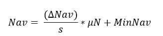
where Δ NAV was the difference between maximum (100) and minimum (30) Nav used in other Alpine landscapes (Seidl et al. 2019), s is the number categories defining poor to rich nutrients (5), μN is the mean value of the nutrient availability for the target forest type and MinNav is the minimum value of available nitrogen (30). This way, we maintained the rate Nav within the typical range of values used in other iLand applications (Seidl et al. 2019, Thom et al. 2022). As we did not have reliable Nav estimates for other land uses, we excluded non-forest areas that were assigned to a default value (e.g., the first quartile of the range distribution) to avoid running into potential crashes during model running. These cells, in any case, do not affect simulation outcomes. Landscape-scale Nav was further adapted during model evaluation to optimize simulated standing volume (refer to section Model evaluation in Results). The final Nav values were implemented in the environment grid at 100 m resolution for the entire project area (Figure S1 in Supplementary material).

Soil carbon and dead organic matter pools

Forest ecosystems play a fundamental role in the global carbon cycle thanks to their capacity to store carbon in soil and deadwood (Fahey et al. 2010, Augusto and Boca 2022). iLand integrates the principles of the ICBM/2N model (Kätterer and Andrén 2001) to model carbon in dead organic matter and soil pools dynamically across the landscape. To do so, the model requires initial estimates for the carbon pools in the form of spatially explicit data about coarse woody debris, litter carbon pools, and soil organic matter. Estimates for standing woody debris (i.e., snags) can also be optionally provided. These estimates are then used as reference values to calculate decomposition rates for litter, downed woody debris, and soil carbon during model evaluation and calibration (described in section on Carbon decomposition rates).

To derive initial carbon pool values in forest areas, we used data from the third Italian National Forest Inventory (hereafter INFC; Gasparini et al. 2022). This information, as is often the case for forest inventories, was available at the point level only. Since there were only a dozen INFC plots inside our study area, to increase the number of data points we selected plots from outside the Venosta study area – yet within the administrative borders of South Tyrol – matching the forest types present in our study area. This resulted in a total of 251 plots containing standing and downed coarse deadwood data. According to the INFC methodological protocol, fine woody debris, litter, and soil carbon pools were measured only in a selection of representative plots, which in our case amounted to 58 plots. Some INFC variables were summed to best match the deadwood and soil parameters needed in iLand (Table S1 in Supplementary). We then imputed INFC plots data to each 100 x 100 m cell according to forest type (layer from Autonomous Province of Bolzano/Bozen 2010), elevation, slope, and aspect derived from the 10-m resolution DEM. Match between points and strata was prioritized if they aligned with all four characteristics. For those strata resulting in zero match with INFC points, we assigned values from similar forest types (e.g., for mixed pine-oak forests we averaged the values of pine and oak forests). For a few strata for which such a procedure was not possible, we used data from Tyrol (Austria), which were used to parametrize another similar forest landscape in the model (Seidl et al. 2019, Marzini et al. 2024). The resulting imputed data were implemented as spatially distributed parameters in the 100 m resolution environment grid for areas covered by forest in the study area (Figure 3).

Figure 3. Distribution of the initial values of soil (som C), litter (young labile C), downed woody debris (young refractory C) and standing woody debris (swd) in the Venosta study area (unit: t ha^-1). 

Climate

Climate clustering

The aim of clustering the study area into climatically homogeneous regions is to reduce the amount of input data processed by the model while retaining the maximum variation across the elevational and topographical gradients. This is one of the most important steps to optimize simulation time in large study areas such as the Venosta. We performed a climate clustering using four climatic variables: minimum temperature, maximum temperature, precipitation sum, and potential solar radiation. Temperature and precipitation gridded data were retrieved as monthly long-term means (1980-2020) as described by Crespi et al. (2021). Solar radiation was derived from monthly raster maps of potential solar radiation corrected by topography and cloud cover at 100 m resolution for the entire South Tyrol province (Tscholl et al. 2021). Temperature and precipitation datasets were resampled from their original 250 m to 100 m resolution using bilinear interpolation.

The cluster analysis was performed by the clustering algorithm CLARA (Kaufman and Rousseeuw 1986) implemented in the R package cluster (Maechler et al. 2019). This algorithm is an extension to k-medoids (PAM) methods to deal with large data sets. Instead of finding medoids for the entire data set, CLARA considers a small sample of the data with a fixed size and applies the PAM algorithm to generate an optimal set of medoids for the sample. The quality of resulting medoids is measured by the average dissimilarity between every object in the entire data set and the medoid of its cluster. The algorithm repeats the sampling and clustering processes a pre-specified number of times to minimize the sampling bias. The Venosta study area is characterized by a complex topography, with a median slope of 25.28° and an average height difference in slope direction between two contiguous 100-m cells of 47.22 m. Assuming a lapse rate of +0.65°C/100m, the average temperature difference between two neighboring cells in the landscape was then 0.30°C, therefore we aimed for 50% of the pixels to have a deviation less than 0.30°C, and ideally, 95% of the pixels to be below the difference of two pixels (0.60°C). We explored an increasing number of climate clusters from a minimum of 100 to a maximum of 1600 (Table S2). To estimate the optimal number of clusters, in addition to assessing deviations from the original dataset, we used the average silhouette method (Rousseeuw 1987). The silhouette width value is a measure of how similar an object is to its own cluster (cohesion) compared to other clusters (separation), ranging from −1 to +1, where a high value indicates that the object is well matched to its own cluster and poorly matched to neighboring clusters. The number of clusters that were more appropriate to capture topography in our region ranged between 500 and 1200 as the silhouette index seemed to be more comparable, with a peak at 800 and 1200 clusters (Figure S2). All tested clusters presented a temperature and precipitation deviation below 1°C and 19 mm. The average silhouette width indicated 800 clusters to be the most representative compared to the others, as they also matched our initial deviation expectations, obtaining 0.18°C and 0.61°C for 50% and 95% of the pixels, respectively (Table S2). We finally selected 800 as the best cluster number for our study area and each 1-ha resource unit was assigned to one climate cluster.

Figure 4. Visualization of the 800 climate clusters in the study area (right) and differences between clustered vs. non-clustered landscape for January minimum temperature (°C) across the landscape and in the form of a histogram (left panels).

Historical climate series (1980-2020)

High-resolution data in forest landscape models are necessary to represent climate variability across complex terrains such as mountain valleys characterized by a high topographic complexity (Torma et al. 2015). iLand requires climate inputs at daily resolution for the following variables: minimum temperature, maximum temperatures, precipitation, global radiation, and vapor pressure deficit (VPD; Figure 5). For the Venosta area, we obtained temperature and precipitation data by extending the high-resolution gridded datasets by Crespi et al. (2021). Series of daily maximum and minimum temperature and precipitation were retrieved at 250-m spatial resolution covering the reference period 1980-2020. Solar radiation daily series were derived from satellite data EUMETSAT, which covered the period 2004-2021 at 4-km resolution[1]. This dataset was compared with other available products with longer series but lower resolutions, such as E-OBS at 12-km resolution (Cornes et al. 2018), and it revealed to be more suitable to capture landscape heterogeneity due to its higher spatial resolution and homogeneous coverage of the domain. EUMETSAT data was downscaled from a 4-km to 250-m grid by a kriging-based approach considering elevation, slope orientation, and steepness as drivers for spatial distribution (Bartkowiak et al. 2022). To consistently cover the entire reference period 1980-2020, solar radiation data before 2004 were reconstructed by following the procedure applied by Leidinger et al. (2018) in the context of the study by Seidl et al. (2019). The relative humidity (RH) needed to derive VPD was retrieved from the E-OBS data set (Cornes et al. 2018). To align it with the resolution of other variables, RH was also downscaled from 12-km to 250-m resolution using a kriging interpolation with elevation as a covariate from the KrigR package (Kusch and Davy 2022).

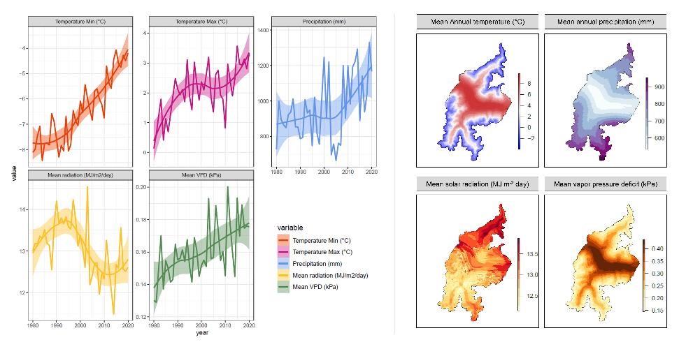
Figure 5. Overview of 1980-2020 reference climate in the Venosta study area. Left panels: time series of climatic variables as landscape means. Lines indicate the average values over the entire area, while ribbons show the 95% confidence interval trend computed with a loess smoothing function. Right panels: spatial distribution across the area of the long-term means (1980-2020) mapped over the 800 climate clusters.

To prevent the interpolation from generating RH values higher than 100%, the quantity √100 − RH was interpolated and transformed back into RH values after the interpolation. Lastly, all five variables covering the historical reference period 1980-2020 at 250-m resolution (Figure 5) were implemented into a SQLite database containing one table per climate cluster linked to each resource unit.

Wind speed and wind topographic pattern

Wind is a crucial factor influencing ecological dynamics in forest ecosystems and it represents the main disturbance agent in European forests (Wohlgemuth et al. 2022, Patacca et al. 2023). Since wind disturbances interacting with bark beetle outbreaks are expected to be amplified under future climate conditions (Seidl et al. 2017, Sommerfeld et al. 2021), it is key to include this disturbance driver into models of forest landscape dynamics. As our aim for future iLand applications in the Venosta study area is to study the potential impacts of wind and bark beetle, we prepared the landscape-specific inputs for the wind disturbance modules and evaluated the ability of the model to simulate wind and bark beetle disturbance (described in section on Model evaluation below). The iLand wind module requires two types of landscape-specific inputs: a topographic exposure modifier map (i.e., topo-modifier) to modulate the effect of topography on the exposure to wind, and a time series of wind events denoting wind speed, wind direction, and storm duration for different days of the year. The occurrence of a wind event on a specific day of the year is relevant because wind risk also depends on the effect of soil freezing and the presence of leaves. We derived the topo-modifier map (Figure S1) using DEM and hill shade mapping products following the approach by Seidl et al. (2014). To derive wind events at the daily resolution, wind direction, and wind speed data were obtained from the Integrated Nowcasting through Comprehensive Analysis (INCA) system (Haiden et al. 2011), which provided hourly wind data at 1-km resolution for Austria and South Tyrol. We downloaded INCA data covering the study area from the first available year (2012) to the end of 2020 and calculated daily values. For each year we identified the maximum gust speed and the associated wind direction. Since we found them to occur mainly during autumn or winter, we determined a wind event for each year as follows: we randomly sampled a day of the year, then we determined the relative wind speed by sampling a random value between i) the range of maximum gust speed for days within autumn and winter; ii) 0 and the maximum gust speed for the days outside autumn and winter. We repeated this procedure for every year to cover the period for model evaluation (see section on Natural disturbances in the Results).

Vegetation

One of the most demanding tasks in forest landscape models is to create a virtual representation of the aboveground vegetation that best resembles the current forest structure and composition. However, it is important that this initial virtual forest landscape is consistent with model logic (e.g., tree placement and competition effects) to avoid unrealistic vegetation development trajectories during the first simulated years. For this reason, but also because species- and size-specific data on live individual trees and regeneration are rarely available in a spatially explicit form, forest landscape models are typically initialized with spin-up simulation routines. This process assimilates the available vegetation data for a specific study area, which is used as a reference, incorporating historical disturbances such as past management interventions that have a long-lasting influence on forest stands (Thom et al. 2018). For the Venosta area, we used data from available forest management plans as reference vegetation state to drive a spin-up procedure to initialize trees in the landscape. Forest management plans were also used to define the spatial setup of the management units and forest stands across the area, in the perspective of simulating forest management strategies under climate change (Mina et al. 2022).

Forest stand data and spatial setup

To prepare our reference vegetation data and to define the spatial setup of the forest management we gathered information from regional forest management plans (FMPs) covering the entire study area (Figure 6). FMPs in South Tyrol are mandatory for publicly owned forests and for private properties larger than 100 ha. They are revised every 10 years and include stand-level information (e.g., stand volume, stand age, species share, site characteristics) and a description of the planned interventions in terms of timber removals in the medium term. For small-scale forest ownerships (< 100 ha), simplified management plans are available (Waldkartei or forest tables) reporting stand information at a lower level of detail. In the Venosta, 92.3% of the forests (11,629 ha) are publicly or collectively owned, with available data from forest management plans (Table S4). Only one section of the landscape (960 ha) fell under small-scale private ownership. For this, we obtained information from ca. 210 forest tables and aggregated them into 36 homogenous stands (with a minimum of 2.5 ha to a maximum of 130 ha), according to similarities in forest structure and composition. In the end, this resulted in the study area being subdivided into a total of 522 forest stands partitioned into 14 management units (Figure 6). Individual stands were assigned with a unique ID code including the unit identifier as the first two digits (e.g., unit 6, stands 21 = StandID 621). For each stand, we compiled stand age, stand volume, and species shares (%), which were used as reference vegetation dataset for model spin-up. Additional data, such as stand mean and dominant height, was available only for a subset of public management units (5 out of 13 units). Height was not included in the reference vegetation dataset for model spin-up but was instead used for model evaluation (see section on Productivity in the Results).

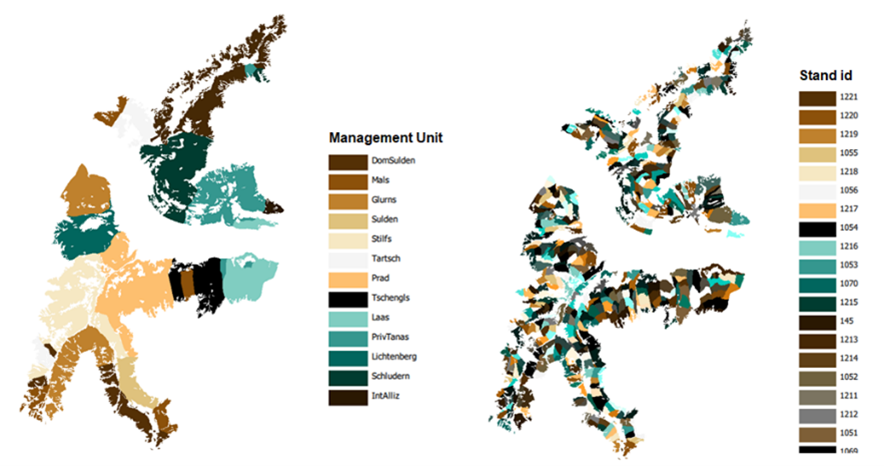
Figure 6. The forest area divided into 14 management units (left) and into the 522 forest stands (right).

Most of the areas outside the stockable area are non-forested (e.g., alpine grassland and rocks above the upper treeline), therefore, are not considered as a source of external seeds that can lead to the establishment and new recruitments. However, in four sections, the stockable area has a border with other forested areas (Figure S3); these were excluded from simulations but had an influence on available light on bordering trees and are potential sources of incoming seeds that may disperse into the stockable area. We defined these areas as our external seed belt. Following the model´s documentation, we split these areas into four sectors, whereas each of them was characterized by a unique species composition. We estimated species composition of each of these four sectors by averaging species shares for the forest stands bordering our stockable area based on data from regional FMPs (additional information in Figure S3).

Spin-up simulation

Current forest landscapes incorporate the legacy of past management and disturbances in their structure and composition (Garbarino and Weisberg 2020). Therefore, model initialization routines such as spin-up simulations – typically performed to assure that initial vegetation states are in line with model-internal processes – should include the effect of past forest management, which is often the most important driver of the current state of forest landscapes, particularly in highly anthropized regions such as the European Alps. In iLand, this is possible via a special spin-up simulation process called legacy spin-up (Thom et al. 2018). This routine consists of a simulation of forest succession dynamics over a long period (e.g., 500-600 years) where simulated forest characteristics at the stand level are constantly compared to the reference vegetation dataset. During this spin-up, an adaptive management regime is applied to each individual stand (e.g., thinning, partial or clear cutting) using the agent-based forest management module (ABE; (Rammer and Seidl 2015). Stands are simulated over multiple rotation periods until conditions closest to the reference data are reached, as defined by a similarity score. This is stored in a temporary database that can be accessed to create a unique landscape “composite” to use as the initial state for simulations (called landscape snapshot).

We followed the procedure described in Thom et al. (2018) and in Seidl et al. (2019), applying the typical management interventions for forests of the European Alps (e.g., planting, tending, thinning, and final cut) to each stand during the spin-up simulation. Spin-up was run over a period of 600 years, during which stand characteristics were iteratively compared with the reference vegetation dataset (described above), and management activities were dynamically adjusted using the ABE module. In the end, we created a landscape snapshot by merging all optimized stands into a single file representing the initial vegetation for the entire study area. This snapshot corresponds to the most up-to-date forest conditions as derived from the forest management plans (see Table S4). However, bark beetle outbreaks starting in 2022 affected forests of the study area, especially in the southern portion where there is a higher share of Norway spruce. Therefore, to achieve a better representation of current forest conditions, we used maps of forest damages due to bark beetle outbreaks derived from Sentinel 2 (Eurac Research 2024) to update the initial vegetation file. Since the available maps indicated stand-replacing damages for the years 2021 until the end of 2023, we removed mature Norway spruce trees directly in the landscape snapshot from those areas overlapping with the resource units covered by pure spruce forests. This way, we created some openings resembling recent bark beetle damages, which could be further analyzed to assess future post-disturbance forest recovery.

Model evaluation

iLand has been extensively evaluated and validated in forest landscapes of Central Europe and in the Alps (Seidl et al. 2019, Honkaniemi et al. 2020, Thom et al. 2022, Dobor et al. 2024). Since our study area was also located in the European Alps, we did not expect the need to re-evaluate internal model parameters and species-specific parameters, which have been recently reviewed and recompiled (Thom et al. 2024). To evaluate model performance, we followed the pattern-oriented modelling approach (Grimm et al. 2005) as typically executed in past model applications. To do so, we tested the ability of the model to: 1) reproduce potential natural vegetation composition; 2) simulate forest productivity; 3) emulate natural disturbances such as wind and bark beetle. For the first test, we ran the model for 1500 years from bare ground, in the absence of natural disturbances or management and assuming unlimited seed availability of all 32 tree species parameterized for Central Europe. After an initial successional sequence, the simulated composition stabilizes into an equilibrium representing the potential natural vegetation (PNV) of the region. We compared this equilibrium to regional forest type mapping products (Autonomous Province of Bolzano/Bozen 2010). To evaluate forest productivity, suitable independent data such as yield tables were not available for our study area. Therefore, we assessed the ability of the model to match reference vegetation data, such as standing volume during the spin-up simulation. We then used standing volume to calibrate model productivity by adapting landscape-level Nav, which was the biophysical parameter with the higher uncertainty rate derived using the concept of soil fertility ranking (see section on Biophysical parameters above). Furthermore, we compared simulated stand mean and dominant height resulting from the landscape snapshot (i.e., the initial state of vegetation generated with model spin-up) with stand height values from regional FMPs. Estimates of mean and dominant stand height were available for stands under public ownership (478 stands, 91.5%). This variable was not used as a reference value to drive the spin-up. Therefore, we used it as an independent variable to evaluate whether the model was able to reproduce dominant height as a proxy of forest productivity. This was evaluated for the selection of stands considering elevation and aspect (section on Productivity in the Results). Lastly, we assessed the ability of the model to reproduce wind and bark beetle disturbances across the study area. For this, we compared the amount of disturbed area to observational data derived from the European forest disturbance map (Senf and Seidl 2021). Since data from the disturbance maps was available from 1986, we ran a 35-year simulation using the landscape snapshot prior to the removal of recent beetle outbreaks at initial vegetation state and historical climate data for the years 1986-2020, activating the bark beetle disturbances module and the wind input and time events data as described in the section on Climate. Since the disturbance maps did not differentiate between wind and beetle damages (Viana-Soto and Senf 2024), we compared the yearly and cumulative damages for both agents. Within the model evaluation, we also assessed parameters related to decomposition rates of the dynamic soil carbon pools and calibrated them using reference values from inventory data as described above. All analyses were conducted in R, version 4.3.0 (R Development Core Team 2023).

RESULTS

Model initialization

The vegetation composition generated by iLand with the legacy spin-up simulation matched well the reference values from forest management plans (Figure 7). No major differences were detected when comparing species composition between simulated and reference conditions, with forests of the study area mainly dominated by Norway spruce, followed by European larch and Swiss stone pine, with regard to species share by volume (Figure 7). Overall, the model slightly overestimated the dominance of Norway spruce and slightly underestimated the presence of silver fir and Swiss stone pine. Other species that are dominant at lower elevational belts (e.g., Scots pine, pubescent oak) were also correctly included, as well as black pine, which is currently present in the area as monospecific plantations close to the south-exposed valley bottom.

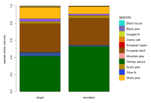
Figure 7. Comparison between reference vegetation dataset (target) and simulated species composition on the study area. Percents of species share were calculated with standing volume.

After removing adult Norway spruce trees in areas hit by recent bark beetle outbreaks (see section on Vegetation), European larch was the species contributing the most in terms of basal area across the study area (37.9%), followed by Norway spruce and Swiss stone pine with 36.6% and 13.1%, respectively. The spatial distribution of the species in the landscape also matched well with the current forest conditions (Figure 8). The southern portion of the study (Stelvio) was mostly dominated by Norway spruce but with a component of silver fir and European larch, with Scots pine towards the valley bottom and Swiss stone pine at subalpine elevation belts (> 1500 m a.s.l.). In the northern portion (Mazia), black pine and pubescent oaks dominated the stands at the valley bottom, while the montane elevation belt (1000-1400 m a.s.l.) was mostly dominated by larch stands, which was promoted by past management for protection and pasture (Pircher and Broll 2014). The internal part of the Mazia valley was instead dominated by European larch and Swiss stone pine, which matches well the reference vegetation dataset from the forest management plans.

 

Figure 8. The initial state of the vegetation as a result of the legacy spin-up routine driven by forest management data. The left panel (a) shows the dominant species, while the right panel (b) indicates stand volume (in m³). Patches in the southern portion of the area more dominated by larch and with a lower standing volume are those in which large spruces were removed following recent bark beetle damages.

Model evaluation

Potential natural vegetation

Forest types emerging from the simulation of potential natural vegetation showed some differences from regional forest-type maps (Figure 9). PNV simulations indicated a higher dominance of Scots pine at montane elevations and a lower occurrence of European larch, which was mainly present in the upper montane to subalpine belts mixed with Swiss stone pine. PNV also showed a higher presence of dwarf mountain pine (Pinus mugo) at the upper treeline, mostly in the northern portion of the study area, which is less abundant in the local forest type mapping (Figure 9). It is important to consider that local forest type maps were developed to show the distribution of the potential natural forest types across the region with a practical viewpoint (Autonomous Province of Bolzano/Bozen 2010). Therefore, although they are useful for describing forest types along elevational belts, they partly embed the effect of past management and disturbances, which we excluded in our PNV simulations. Despite the presence of a higher number of species at the end of the PNV simulation, the dominant species along the elevational belts were comparable to the reference forest types. This indicated that iLand was able to replicate satisfactorily the environmental gradient and reproduce differences in forest conditions at different elevations in our study area.  

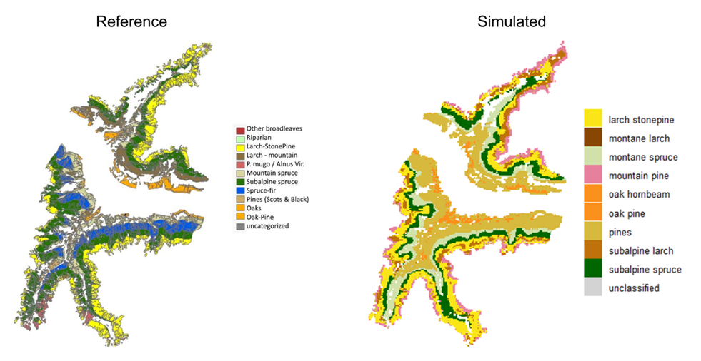
Figure 9. Comparison between local forest type maps (left) and simulated forest types (right) obtained at the end of the 1500-year simulation of potential natural vegetation. Forest types from simulations were defined with tree species shares (basal area) from iLand´s outputs following the descriptions from the report of the forest types for South Tyrol.

The successional sequence in the PNV simulation differed strongly between elevational belts (Figure 10). At low elevations (<1200 m a.s.l.), Scots pine, oaks and black pine showed the highest dominance among species, with a total basal area of about 20-25 m²/ha. This is realistic given that productivity in forests at the Venosta Valley bottom is generally low because limited by water availability. With increasing elevation, the potential forest becomes more dominated by Norway spruce, with productivity increasing (> 40 m²/ha basal area) due to higher water availability thanks to more abundant annual precipitation (see distribution of annual precipitation in Figure 5). Above 1800 m a.s.l. until the upper treeline, European larch and Swiss stone pine gained abundance, which is also plausible as these are the two species that typically dominate the subalpine elevational belt in this region. European beech (Fagus sylvatica), which was included in the list of potential species, never gained dominance at any elevational belt and was even absent in the montane belt (Figure 10). The development of basal area averaged across the entire study area is shown in Figure S4.

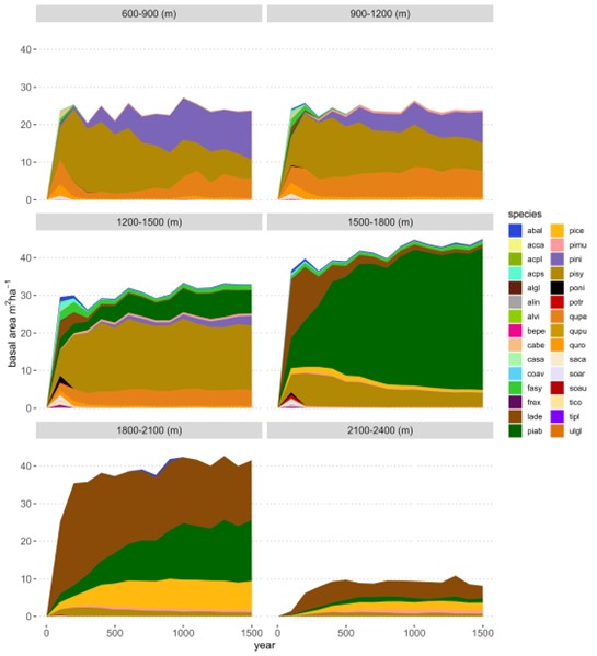
Figure 10.  Basal area development in the PNV simulation under historical climate starting from the bare ground over the time period of 1500 years. Panels show basal area for different elevation classes (every 300 m). Species codes and names are reported in Table S3.

Productivity

An initial comparison of simulated standing volume from model spin-up showed a general overestimation of this variable for forests of different age classes (Figure 11a). The simulated standing volume was in the range of 500±100 m³/ha, while the mean target stand volume was about 250±100 m³/ha (Figure 11b). This was likely due to overestimated values of Nav, which could be derived only with an indirect method (see section on Biophysical parameters). Therefore, we reduced the overall range of available nitrogen of all resource units in subsequent steps (90^th, 80^th, 75^th percentile of initially estimated values), re-ran the model spin-up procedure and compared again with target stand volumes. In the end, standing volume simulated with Nav values capped to the 75^th percentile (i.e., -25% of Nav) yielded the best comparison with reference volume data, both at the landscape level and for the different age classes (Figure 11 c, b).

Figure 11. Comparison of productivity (mean standing volume) between simulated and reference values. Upper panels (a, b) show the first comparison with the initial estimates of Nav, and lower panels (b, c) show the final comparison with adjusted Nav at the landscape level.

The comparison of simulated and observed stand mean and dominant height indicated a general underestimation of simulated tree height at the landscape level (Figure 12). This underestimation was more evident for stands in the montane elevational belt (1300-1600 m a.s.l.) but less apparent at lower and upper elevations. Despite this underestimation, we decided not to adjust further model parameters, particularly considering that standing volume showed a good match with empirical observations and that observed stand height from regional FMPs are also subject to uncertainty, given that they are mostly derived from ocular estimations rather than in situ measurements. Regardless, the simulated dominant height was positively correlated with observations (r=0.31), and the trend of the simulated dominant stand height along elevation and aspect gradients was in line with the trend of observed values (Figure 12).

Figure 12. Evaluation of forest productivity with dominant stand height. Left panel Comparison of simulated (95^th percentile of tree height) and observed dominant stand height from FMPs. Right panels show simulated vs observed dominant height along the elevational and aspect gradients. Stand height in FMPs was not available for individual species but only aggregated at stand level.

Natural disturbances

The total disturbed area by wind and bark beetle over the simulated period 1986-2020 matched very well with respective observations (Figure 13). Compared to the European Forest Disturbance Maps (EFDM) data by Senf and Seidl (2021), iLand underestimated cumulative disturbances only by 6.1% (Figure 13b). Although the total disturbance impact was very close to observations, some differences could be detected when comparing observations with annual simulation outputs (Figure 13a). The observed impact of both wind and beetles was higher in some years (1989, 1995, 2001), and the model was not able to replicate the magnitude of cumulative damages of these two agents in the study area in those years; instead, it simulated more frequent wind and beetle disturbances during the entire evaluation period. This is likely due to the occurrence of small-scale windthrow events in the study area that could not be replicated with the wind input data series (refer to section on Climate).

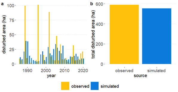
Figure 13. a) Time series (1986-2020) of disturbance impact (disturbed area in ha) from observations (EFDM data) and simulation outputs. Disturbances include both bark beetle and wind, as the EFDA maps did not distinguish individual agents. b) comparison of the cumulated disturbed area from bark beetle and wind between EFDM observations and simulations during the period 1986-2020.

Carbon decomposition rates

After running the first spin-up simulation, soil and deadwood carbon pools generated by iLand (Table S1) were compared with initial carbon pool values derived from forest inventory (refer to the section on Biophysical parameters). This is shown in Figure 14a, where it can be observed that simulated downed woody debris (young refractory C) and standing deadwood (snag C) values trends followed the reference values but with a slight underestimation. Simulated soil (soil C) and litter (young labile) carbon, instead, were simulated to be much lower than reference values. We re-run the model spin-up with adjusted decomposition rates for young labile, young refractory and soil organic matter carbon pools, assuming a uniform humification rate of 0.25, as recommended in the model documentation. After calibration (Figure 14b), simulated soil and litter carbon values stabilized close to reference data of about 100 t/ha and 12.5 t/ha, respectively. Downed woody debris and snags changed only slightly after calibration, stabilizing to much lower values yet close to reference data.  

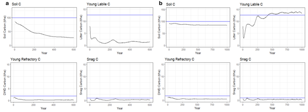
Figure 14. Development of the carbon pools needed in iLand over a) the first spin-up, and b) over the second spin-up after the adjustment of the decomposition rates. Blue lines indicate the reference carbon values averaged across the landscape based on INFC data. Beware of the different scales of the y-axis for the different pools. 

DISCUSSION

Forest landscape models are becoming important tools to investigate forest ecosystems dynamics under changing conditions and future scenarios. However, the ability of a model to reproduce forest dynamics depends largely on the quality of input data (Reyer et al. 2016). Moreover, the evaluation of main simulation processes is fundamental to improving model reliability, especially given the increasing complexity of these tools (Bugmann and Seidl 2022). Although there is a strong willingness to apply these tools in forests worldwide, users often encounter challenges with model parameterization, exacerbated by the lack of suitable spatial data and the absence of comparable examples for establishing new study areas. These challenges, along with the significant investment of time needed to prepare and set up a new study area, greatly limit the applicability of such tools in supporting forest management. iLand has a user-friendly interface and extensive documentation that helps modellers and professionals to establish new applications. Despite this, preparing all the required input data to set up new study regions, including model initialization and evaluation, remains a strenuous and time-consuming task. For this reason, in the present study we documented the overall processes and the methodological steps needed to initialize a large landscape in iLand, with the aim of promoting its application in other study areas in the Italian Alps and beyond. 

Regarding model initialization, we applied a spin-up simulation procedure to obtain the most representative condition of the current forest, using reference data from forest management plans after characterizing the project area with biophysical and climate conditions. Results from model spin-up in terms of species composition showed a good match with reference data, indicating that the internal dynamics of the model are able to reproduce in a satisfactory manner the differences in forest composition along the large environmental gradient of the area. The simulated landscape had, however, a slightly overestimated presence of Norway spruce compared to reference vegetation data, whereas Swiss stone pine and silver fir shares were somewhat underestimated. These results are consistent with other studies in mountain landscapes parametrized in iLand (Thom et al. 2018, Seidl et al. 2019), where Norway spruce was found to be more dominant in the simulated landscape compared to reference observations. This might be related to the parameterization of this species in the model, with Norway spruce being more competitive under certain climate conditions, or to the different ecological behavior of this species in the south of the Alps due to the genetic differentiation of the local population (Di Pierro et al. 2017). Since species parameters for Norway spruce in iLand are categorized to have a high level of confidence (Thom et al. 2024), we decided not to proceed with further calibration efforts at the species level. However, we also must acknowledge some limitations in our reference vegetation dataset. We could only gather data of forest composition, volume and age aggregated at stand level, as the number of forest inventory plots with individual-tree data was not enough to perform a spatial imputation on the most common forest types covering the entire area (as shown in other studies like Duveneck et al. 2015, Mina et al. 2021). Also, we are aware that for a number of stands, these data were derived from ocular estimates from the forest service personnel rather than from structured and spatially consistent measurements. Additionally, we did not use landscape-scale canopy height data to refine tree positions and canopy gaps and to better evaluate tree dominant height because the latest airborne-based LiDAR data was not recent enough (2007). Since airborne LiDAR data and other fine-resolution remote sensing products are becoming more and more accessible, our representation of initial vegetation could be improved in the near future. Another limitation that might have slightly affected model performance was the source of climate data. Parameterizing a study area with a single data source for all variables would be preferable since this would ensure the overall consistency among variables. However, the procedures we adopted to align and resample the available gridded climate data from different products can be an adequate alternative and easily applicable to any other domain. Despite these limitations in the available vegetation and other input data, we believe that the initialized forest landscape is well representative of the initial vegetation and biophysical conditions of the study area, and can be used as a starting point for modelling future forest landscape development under different scenarios (Albrich et al. 2020a, Mina et al. 2022, Thom et al. 2022).

Concerning model evaluation, we assessed the model's ability to reproduce forest conditions following a pattern-oriented procedure (Grimm et al. 2005) as recommended in previous iLand applications (Seidl et al. 2019, Dobor et al. 2024). This methodology has been proven to be useful to observe different patterns at various hierarchical organization levels for assessing the robustness of simulation models (Gallagher et al. 2021). The emergent vegetation simulated in the absence of natural and anthropic disturbances (PNV) was in line with the expected late-seral tree species composition along our environmental gradient. The forest categories dominating the study area at the simulated climax were plausible given the climatic limitations, with oaks- and pine-dominated forests covering the lower montane elevational belt, transitioning to Norway spruce and larch-stone pine forests towards the upper montane to subalpine elevations (Figure 9). Compared to other landscapes parameterized in iLand (Albrich et al. 2018, Seidl et al. 2019, Thom et al. 2022, Dobor et al. 2024), our study area is the first one located in the south of the European Alps, and the first example of a landscape sited within a dry inner-alpine valley where species composition and tree growth at the valley bottom are strongly limited by water availability (Rigling et al. 2013, Obojes et al. 2024). It is interesting to note that, European beech (Fagus sylvatica) – which was included in the list of potential species and often simulated as one of the main climax species (Dobor et al. 2024) – was absent at all elevational belts (Figure 10). This is coherent with observations since beech is practically absent in the Venosta Valley because of insufficient relative humidity and due to a too-continental climate preventing its establishment and growth (Zischg et al. 2019). Our PNV simulations indicate that iLand was able to capture the environmental constraints driving regeneration dynamics and inter-specific competition in landscapes of the southern edge of the European Alps. Our comparison with regional-type mapping, however, should be taken cautiously for two reasons. First, the categorization of the forest into forest types (see Figure 9) could not be replicated precisely, as no guidelines about the criteria used for realizing the forest categories present in the regional maps were available (Autonomous Province of Bolzano/Bozen 2010). Therefore, the forest categories that we derived using iLand outputs could have been different if we chose different thresholds of basal area of the individual species to reclassify the map. Second, we cannot be sure that the regional forest-type maps really describe the potential natural vegetation of the province since, among other cartographic products, current vegetation maps were also used as a starting point for building these reference maps. Despite this limitation in reference data, iLand reproduced potential natural vegetation very close to expectations for our study area and in line with other simulation studies for Central European and Alpine landscapes (Thom et al. 2018, Seidl et al. 2019).

As recommended by model developers, evaluation tests vary among landscapes due to the availability and the limitation of reference data in each study area (Rammer et al. 2024). In our case, we followed an iterative approach when evaluating stand productivity, knowing that our initial estimates of available nitrogen – an important biophysical property driving tree growth (Rennenberg and Dannenmann 2015) – were highly uncertain due to the lack of high-resolution spatial data for this variable. We therefore used standing volume as comparison data to calibrate available nitrogen levels at the landscape level and subsequently evaluated forest productivity with independent observations of stand dominant height. We are aware that this evaluation process could be improved if local forest inventories and yield tables data were available. However, our evaluation and calibration method employs data that are typically available in local forest management plans or openly-available remote sensing products and can therefore be applied in regions that lack long-term inventory series (e.g.,  Bychkov and Popova 2023).

Evaluation tests also depend on the type of application that is expected to be carried out after the parameterization of the study area. In our case, our aim for future studies is to apply iLand in the Venosta area to assess the vulnerability of these forests to climate-change-induced disturbances but also to investigate the future carbon sink potential of Alpine forests. For this reason, we tested the ability of the model to capture the most important disturbances occurring in the Alps and evaluated the carbon cycling module. Evaluating the model´s capability to emulate natural disturbances is key when models include interactions between disturbance types, such as in our case between wind and bark beetle (Sturtevant and Fortin 2021). Independent comparison data of forest disturbances are often available for very short time series, which most of the time limits the ability to fully evaluate the model, even when using the pattern-based approach. Our evaluation results showed that the model was able to reproduce the cumulative effects of wind and bark beetle disturbances regime in forests of the Italian Alps very well, but it was less precise to capture yearly variation of disturbance intensity. This was somewhat expected since the wind input data was designed to represent wind patterns for the historical reference period rather than to replicate precisely the intensity of windstorms that occurred during recent years. Analogous results were shown by Thom et al. (2022), where the model reproduced very well cumulative disturbed areas against observations, but it was less precise to replicate annual disturbances. Also, disturbance maps used as independent observations often report cumulative damages from multiple disturbance agents (Senf and Seidl 2021) although more recent mapping products separate logging and fire disturbances from wind and beetles (Viana Soto and Senf 2024). In our case, disturbance maps combined wind and bark beetle damages; therefore, we could not compare the damages for single disturbance agents. Longer series of wind disturbance data would be ideal, but remote sensing products typically cover only a few decades. However, since the aim of dynamic landscape models like iLand is to capture the impact of disturbance regimes in the long term – and not to exactly replicate a specific disturbance event – our evaluation can be considered satisfactory.

Regarding forest carbon pools, modelling changes in carbon fluxes and storage across forested landscapes has been challenging due to the intricate interactions between landscape structure and ecosystem processes (Chen et al. 2014). Only a few forest landscape models, including iLand, explicitly integrate carbon dynamics (Dymond et al. 2012, Albrich et al. 2023, Lucash et al. 2023), but often require more parameters and intense calibration exercises for soil pools initialization (Dymond et al. 2016). Forest carbon pools data is rarely available as spatially continuous datasets, as was the case for our study area, where we had to perform a spatial imputation using inventory data from sampling points distributed also outside our project area. Therefore, we acknowledge that the data used might not be fully representative of the variation range of carbon pools within our study area, and relative uncertainties might be further amplified during the scaling processes, as shown in previous studies (Vanguelova et al. 2016). Despite these limitations, we presented a methodology that can be easily replicated in other landscapes in Italy, as we made the best use of publicly available data from the Italian National Forest Inventory (Gasparini et al. 2022). Moreover, these data showed also to be comparable with values observed in other forest areas of the Alpine region (Prietzel and Christophel 2014, De Vos et al. 2015, Canedoli et al. 2020), confirming the plausibility of the gathered information although derived from sample plots within a larger region (e.g., South Tyrol) than the project area. Despite having used data from different sources, our results improved the robustness of the initialized landscape in iLand, which can be used to run future investigations on carbon cycling dynamics to study forest mitigation potential to climate change under a suite of different scenarios.

Despite some caveats mentioned above, the iLand model showed good potential for applications in the Italian Alps. The model can be now applied in the Venosta study area to investigate forest development under different management, disturbances and climate scenarios, which would be useful to inform decision-makers in forest policy and ecosystem management (e.g., Maxwell et al. 2020, Mina et al. 2022). As future avenues, given the increasing availability of data from individual tree detection laser scanners at large-scale (Hyyppä et al. 2024), such models can make use of more accurate reference data to initialize current vegetation. This, however, should be considered with caution, as higher resolution initialization data also requires even more complex data preparation routines. The forest modelling community should therefore work on developing ways to fully utilize the newly available data wealth efficiently for model initialization (Keane et al. 2015, Furniss et al. 2022). Another prospect for future development is to better link the outputs of forest models with realistic visualization of the forests for better communication with stakeholders (Huang et al. 2021). Building digital twins of forests and applying virtual reality tools using data generated from forest models could better support forest management by demonstrating the impact of silvicultural interventions on forest structure at the landscape scale (Holm and Schweier 2024). An important aspect to consider, particularly if models are meant to be operated by managers and stakeholders, is model choice. Complex process-based landscape models like iLand are indeed valuable for exploring landscape levels dynamics under climate change and disturbances over the longer term but are not meant to provide operational information on a stand-level (Shifley et al. 2017). Therefore, for shorter-term management planning and more basic applications in forestry other models with less heavy data requirements and simpler disturbance risk implementation may be more suitable (Hillebrand et al. 2023, Blattert et al. 2024). Lastly, although process-based landscape models like iLand need a lot of information for setup and testing, flexible data processing and integration methods, as shown in this study, allow the use of various data types and resolutions. This makes these models a powerful, widely applicable tool for exploring the interactions of forest dynamics, climate, disturbances and management.

CONFLICTS OF INTEREST

The authors confirm there are no conflicts of interest.

ACKNOWLEDGEMENTS

Marco Mina and Sebastian Marzini acknowledge funding from the European Union’s Horizon 2020 research and innovation program under the Marie Skłodowska-Curie framework (grant n.891671, project REINFORCE) and the European Interreg IT-CH project “MAP-Rezia” (ID 0200061, program 2021-2027). Katharina Albrich was partially supported by funding from the Finnish Ministry of Agriculture and Forestry (“Catch the Carbon” initiative, project FOSTER, project number VN/28654/2020) and the Academy of Finland (project MULTIRISK, grant numbers 353263 and 353264). We thank the Forest Planning Office of the Provincial Forest Services of South Tyrol for providing forest management data for parameterizing the model on the study area, in particular Marco Pietrogiovanna and Hannes Markart. The authors thank Thomas Marsoner for the help in preparing some spatial input data, Erich Tasser and Nikolaus Obojes for general advice on the choice of the study area, and Werner Rammer for supporting the model calibration.

DATA AVAILABILITY

Data that supports the finding of this study are archived in Zenodo at https://doi.org/10.5281/zenodo.14886673. The iLand model, including documentation and the source code, is freely available at https://iland-model.org/ under the GNU General Public License.

REFERENCES CITED

 Albrich K, Rammer W, Seidl R. 2020a. Climate change causes critical transitions and irreversible alterations of mountain forests. Global Change Biology 26:4013-4027. https://doi.org/10.1111/gcb.15118

Albrich K, Rammer W, Thom D, Seidl R. 2018. Trade-offs between temporal stability and level of forest ecosystem services provisioning under climate change. Ecological Applications 28:1884-1896. https://doi.org/10.1002/eap.1785

Albrich K, Rammer W, Turner MG, Ratajczak Z, Braziunas KH, Hansen WD, Seidl R. 2020b. Simulating forest resilience: A review. Global Ecology and Biogeography 29:2082-2096. https://doi.org/10.1111/geb.13197

Albrich K, Seidl R, Rammer W, Thom D, Fassnacht F. 2023. From sink to source: changing climate and disturbance regimes could tip the 21st century carbon balance of an unmanaged mountain forest landscape. Forestry 96:399-409. https://doi.org/10.1093/forestry/cpac022

Augusto L, Boca A. 2022. Tree functional traits, forest biomass, and tree species diversity interact with site properties to drive forest soil carbon. Nature Communications 13:1097. https://doi.org/10.1038/s41467-022-28748-0

Autonomous Province of Bolzano/Bozen. 2010. Waldtypisierung Südtirol - Tipologie Forestali dell'Alto Adige - Forest Types of South Tyrol. Bolzano/Bozen https://www.provincia.bz.it/agricoltura-foreste/bosco-legno-malghe/studi-progetti/tipologie-forestali-in-alto-adige.asp accessed on 13.05.2024.

Bartkowiak P, Castelli M, Crespi A, Niedrist G, Zanotelli D, Colombo R, Notarnicola C. 2022. Land surface temperature reconstruction under long-term cloudy-sky conditions at 250 m spatial resolution: case study of Vinschgau/Venosta Valley in the European Alps. IEEE Journal of Selected Topics in Applied Earth Observations and Remote Sensing 15:2037-2057. https://doi.org/10.1109/JSTARS.2022.3147356

Blattert C, Mutterer S, Thrippleton T, Diaci J, Fidej G, Bont LG, Schweier J. 2024. Managing European Alpine forests with close-to-nature forestry to improve climate change mitigation and multifunctionality. Ecological Indicators 165:112154. https://doi.org/10.1016/j.ecolind.2024.112154

Bonan GB. 2008. Forests and climate change: Forcings, feedbacks, and the climate benefits of forests. Science 320:1444-1449. https://doi.org/10.1126/science.1155121

Bosela M, Merganičová K, Torresan C, Cherubini P, Fabrika M, Heinze B, Höhn M, Kašanin-Grubin M, Klopčič M,  Mészáros I. 2022. Modelling future growth of mountain forests under changing environments. Climate-Smart Forestry in Mountain Regions 223. https://doi.org/10.1007/978-3-030-80767-2_7

Bugmann H, Seidl R. 2022. The evolution, complexity and diversity of models of long-term forest dynamics. Journal of Ecology 110:2288-2307. https://doi.org/10.1111/1365-2745.13989

Bychkov I, Popova A. 2023. Forest landscape model initialization with remotely sensed-based open-source databases in the absence of inventory data. Forests 14:1995. https://doi.org/10.3390/f14101995

Canedoli C, Ferrè C, Abu El Khair D, Comolli R, Liga C, Mazzucchelli F, Proietto A, Rota N, Colombo G, Bassano B, Viterbi R, Padoa-Schioppa E. 2020. Evaluation of ecosystem services in a protected mountain area: Soil organic carbon stock and biodiversity in alpine forests and grasslands. Ecosystem Services 44:101135. https://doi.org/10.1016/j.ecoser.2020.101135

Chen J, John R, Sun G, McNulty S, Noormets A, Xiao J, Turner MG, Franklin JF. 2014. Carbon fluxes and storage in forests and landscapes. Pages 139-166 in J. C. Azevedo, A. H. Perera, and M. A. Pinto, editors. Forest landscapes and global change: Challenges for research and management. Springer New York, New York, NY. https://doi.org/10.1007/978-1-4939-0953-7_6

Cornes RC, van der Schrier G, van den Besselaar EJM, Jones PD. 2018. An ensemble version of the E-OBS temperature and precipitation data sets. Journal of Geophysical Research: Atmospheres 123:9391-9409. https://doi.org/10.1029/2017JD028200

Crespi A, Matiu M, Bertoldi G, Petitta M, Zebisch M. 2021. A high-resolution gridded dataset of daily temperature and precipitation records (1980-2018) for Trentino-South Tyrol (north-eastern Italian Alps). Earth Syst. Sci. Data 13:2801-2818. https://doi.org/10.5194/essd-13-2801-2021

De Vos B, Cools N, Ilvesniemi H, Vesterdal L, Vanguelova E, Carnicelli S. 2015. Benchmark values for forest soil carbon stocks in Europe: Results from a large scale forest soil survey. Geoderma 251-252:33-46. https://doi.org/10.1016/j.geoderma.2015.03.008

Di Pierro EA, Mosca E, González-Martínez SC, Binelli G, Neale DB, La Porta N. 2017. Adaptive variation in natural Alpine populations of Norway spruce (Picea abies [L.] Karst) at regional scale: Landscape features and altitudinal gradient effects. Forest Ecology and Management 405:350-359. https://doi.org/10.1016/j.foreco.2017.09.045

Dobor L, Baldo M, Bílek L, Barka I, Máliš F, Štěpánek P, Hlásny T. 2024. The interacting effect of climate change and herbivory can trigger large-scale transformations of European temperate forests. Global Change Biology 30:e17194. https://doi.org/10.1111/gcb.17194

Dollinger C, Rammer W, Suzuki KF, Braziunas KH, Keller TT, Kobayashi Y, Mohr J, Mori AS, Turner MG, Seidl R. 2024. Beyond resilience: Responses to changing climate and disturbance regimes in temperate forest landscapes across the Northern Hemisphere. Global Change Biology 30:e17468. https://doi.org/10.1111/gcb.17468

Duveneck MJ, Thompson JR, Wilson BT. 2015. An imputed forest composition map for New England screened by species range boundaries. Forest Ecology and Management 347:107-115. https://doi.org/10.1016/j.foreco.2015.03.016

Dymond CC, Beukema S, Nitschke CR, Coates KD, Scheller RM. 2016. Carbon sequestration in managed temperate coniferous forests under climate change. Biogeosciences Discussions 12:20283-20321. https://doi.org/10.5194/bgd-12-20283-2015

Dymond CC, Scheller RM, Beukema S. 2012. A new model for simulating climate change and carbon dynamics in forested landscapes. Ecosystems Management 13:1-2. https://doi.org/10.22230/jem.2012v13n2a209

EEA. 2018. Copernicus High Resolution Layer Forest Type. Copernicus Land Monitoring Service, European Environment Agency (EEA). https://doi.org/10.2909/59b0620c-7bb4-4c82-b3ce-f16715573137.

Ehrenfeld JG, Ravit B, Elgersma K. 2005. Feedback in the plant-soil system. Annual Review of Environment and Resources 30:75-115. https://doi.org/10.1146/annurev.energy.30.050504.144212

Eurac Research. 2024. Ips typographus annual progression maps. Autonomous Province of Bolzano/Bozen. GeoBrowser MapView South Tyrol. Available at: https://mapview.civis.bz.it/.

Fahey TJ, Woodbury PB, Battles JJ, Goodale CL, Hamburg SP, Ollinger SV, Woodall CW. 2010. Forest carbon storage: ecology, management, and policy. Frontiers in Ecology and the Environment 8:245-252. https://doi.org/10.1890/080169

Fontes L, Bontemps JD, Bugmann H, Van Oijen M, Gracia C, Kramer K, Lindner M, Rotzer T, Skovsgaard JP. 2010. Models for supporting forest management in a changing environment. Forest Systems 19:8-29. https://doi.org/10.5424/fs/201019S-9315

Forzieri G, Girardello M, Ceccherini G, Spinoni J, Feyen L, Hartmann H, Beck PSA, Camps-Valls G, Chirici G, Mauri A, Cescatti A. 2021. Emergent vulnerability to climate-driven disturbances in European forests. Nat Commun 12:1081. https://doi.org/10.1038/s41467-021-21399-7

Furniss TJ, Hessburg PF, Povak NA, Salter RB, Wigmosta MS. 2022. Predicting future patterns, processes, and their interactions: Benchmark calibration and validation procedures for forest landscape models. Ecological Modelling 473:110099. https://doi.org/10.1016/j.ecolmodel.2022.110099

Gallagher CA, Chudzinska M, Larsen-Gray A, Pollock CJ, Sells SN, White PJC, Berger U. 2021. From theory to practice in pattern-oriented modelling: identifying and using empirical patterns in predictive models. Biological Reviews 96:1868-1888. https://doi.org/10.1111/brv.12729

Garbarino M, Weisberg PJ. 2020. Land-use legacies and forest change. Landscape Ecology 35:2641-2644. https://doi.org/10.1007/s10980-020-01143-0

Gasparini P, Di Cosmo L, Floris A, De Laurentis D. 2022. Italian National Forest Inventory-methods and results of the third survey: Inventario Nazionale delle Foreste e dei Serbatoi Forestali di Carbonio-Metodi e Risultati della Terza Indagine. Springer Nature. https://doi.org/10.1007/978-3-030-98678-0

Gret-Regamey A, Brunner SH, Kienast F. 2012. Mountain ecosystem services: who cares? Mountain Research and Development 32:S23-S34. https://doi.org/10.1659/MRD-JOURNAL-D-10-00115.S1

Grimm V, Revilla E, Berger U, Jeltsch F, Mooij WM, Railsback SF, Thulke HH, Weiner J, Wiegand T, DeAngelis DL. 2005. Pattern-oriented modeling of agent-based complex systems: lessons from ecology. Science 310:987-991. https://doi.org/10.1126/science.1116681

Grünig M, Seidl R, Senf C. 2023. Increasing aridity causes larger and more severe forest fires across Europe. Global Change Biology 29:1648-1659. https://doi.org/10.1111/gcb.16547

Gustafson EJ. 2013. When relationships estimated in the past cannot be used to predict the future: using mechanistic models to predict landscape ecological dynamics in a changing world. Landscape Ecology 28:1429-1437. https://doi.org/10.1007/s10980-013-9927-4

Haiden T, Kann A, Wittmann C, Pistotnik G, Bica B, Gruber C. 2011. The integrated nowcasting through comprehensive analysis (INCA) system and its validation over the Eastern Alpine Region. Weather and Forecasting 26:166-183. https://doi.org/10.1175/2010WAF2222451.1

Hillebrand L, Marzini S, Crespi A, Hiltner U, Mina M. 2023. Contrasting impacts of climate change on protection forests of the Italian Alps. Frontiers in Forests and Global Change 6. https://doi.org/10.3389/ffgc.2023.1240235

Hof AR, Mina M, Mairota P, Klopčič M, Koivula M, Brůna J, Leitinger G, Vacchiano G. 2024. A perspective on the need for integrated frameworks linking species distribution and dynamic forest landscape models across spatial scales. Frontiers in Ecology and Evolution 12. https://doi.org/10.3389/fevo.2024.1112712

Holland TG, Evans SG, Long JW, Maxwell C, Scheller RM, Potts MD. 2022. The management costs of alternative forest management strategies in the Lake Tahoe Basin. Ecology and Society 27. https://doi.org/10.5751/ES-13481-270443

Holm S, Schweier J. 2024. Virtual forests for decision support and stakeholder communication. Environmental Modelling & Software 180:106159. https://doi.org/10.1016/j.envsoft.2024.106159

Holzer D, Bödeker K, Rammer W, Knoke T. 2024. Evaluating dynamic tree-species-shifting and height development caused by ungulate browsing in forest regeneration using a process-based modeling approach. Ecological Modelling 493:110741. https://doi.org/10.1016/j.ecolmodel.2024.110741

Honkaniemi J, Rammer W, Seidl R. 2020. Norway spruce at the trailing edge: the effect of landscape configuration and composition on climate resilience. Landscape Ecology 35:591-606. https://doi.org/10.1007/s10980-019-00964-y

Huang J, Lucash MS, Scheller RM, Klippel A. 2021. Walking through the forests of the future: using data-driven virtual reality to visualize forests under climate change. International Journal of Geographical Information Science 35:1155-1178. https://doi.org/10.1080/13658816.2020.1830997

Hyyppä M, Turppa T, Hyyti H, Yu X, Handolin H, Kukko A, Hyyppä J, Virtanen JP. 2024. Concepts towards nation-wide individual tree data and virtual forests. ISPRS International Journal of Geo-Information 13:424. https://doi.org/10.3390/ijgi13120424

ITMN. 2025. International Tree Mortality Network - Towards a global understanding of tree mortality. New Phytologist n/a.

Kaarakka L, Cornett M, Domke G, Ontl T, Dee LE. 2021. Improved forest management as a natural climate solution: A review. Ecological Solutions and Evidence 2:e12090. https://doi.org/10.1002/2688-8319.12090

Kätterer T, Andrén O. 2001. The ICBM family of analytically solved models of soil carbon, nitrogen and microbial biomass dynamics - descriptions and application examples. Ecological Modelling 136:191-207. https://doi.org/10.1016/S0304-3800(00)00420-8

Kaufman L, Rousseeuw PJ. 1986. Clustering large datasets. Pages 425-437 in E. S. Gelsema and L. N. Kanal, editors. Pattern Recognition in Practice. Elsevier, Amsterdam. https://doi.org/10.1016/B978-0-444-87877-9.50039-X

Keane RE, McKenzie D, Falk DA, Smithwick EAH, Miller C, Kellogg L-KB. 2015. Representing climate, disturbance, and vegetation interactions in landscape models. Ecological Modelling 309-310:33-47. https://doi.org/10.1016/j.ecolmodel.2015.04.009

Kirchen G, Calvaruso C, Granier A, Redon P-O, Van der Heijden G, Bréda N, Turpault M-P. 2017. Local soil type variability controls the water budget and stand productivity in a beech forest. Forest Ecology and Management 390:89-103. https://doi.org/10.1016/j.foreco.2016.12.024

Kusch E, Davy R. 2022. KrigR-a tool for downloading and statistically downscaling climate reanalysis data. Environmental Research Letters 17:024005. https://doi.org/10.1088/1748-9326/ac48b3

Landsberg JJ, Waring RH. 1997. A generalised model of forest productivity using simplified concepts of radiation-use efficiency, carbon balance and partitioning. Forest Ecology and Management 95:209-228. https://doi.org/10.1016/S0378-1127(97)00026-1

Leidinger D, Formayer H, Nadeem I, Frisch-Niggemayer A. 2018. Localization of climate-data for Stubai Valley: HiReSt. Institute of Meteorology (BOKU-Met), University of Natural Resources and Life Sciences, Vienna.

Lucash MS, Marshall AM, Weiss SA, McNabb JW, Nicolsky DJ, Flerchinger GN, Link TE, Vogel JG, Scheller RM, Abramoff RZ, Romanovsky VE. 2023. Burning trees in frozen soil: Simulating fire, vegetation, soil, and hydrology in the boreal forests of Alaska. Ecological Modelling 481:110367. https://doi.org/10.1016/j.ecolmodel.2023.110367

Maechler M, Rousseeuw P, Struyf A, Hubert M, Hornik K. 2019. Cluster: cluster analysis basics and extensions. R package version 2.1.1.

Marzini S, Tasser E, Wellstein C, Albrich K, Rammer W, Mina M. 2024. Future expansion of alpine forest-grassland ecotone under land-use and climate change. Researchsquare (Preprint). https://doi.org/10.21203/rs.3.rs-4789034/v1

Maxwell CJ, Serra-Diaz JM, Scheller RM, Thompson JR. 2020. Co-designed management scenarios shape the responses of seasonally dry forests to changing climate and fire regimes. Journal of Applied Ecology 57:1328-1340. https://doi.org/10.1111/1365-2664.13630

McDowell NG, Allen CD, Anderson-Teixeira K, Aukema BH, Bond-Lamberty B, Chini L, Clark JS, Dietze M, Grossiord C, Hanbury-Brown A, Hurtt GC, Jackson RB, Johnson DJ, Kueppers L, Lichstein JW, Ogle K, Poulter B, Pugh TAM, Seidl R, Turner MG, et al. 2020. Pervasive shifts in forest dynamics in a changing world. Science 368:eaaz9463. https://doi.org/10.1126/science.aaz9463

Millar CI, Stephenson NL. 2015. Temperate forest health in an era of emerging megadisturbance. Science 349:823-826. https://doi.org/10.1126/science.aaa9933

Mina M, Bugmann H, Cordonnier T, Irauschek F, Klopcic M, Pardos M, Cailleret M. 2017. Future ecosystem services from European mountain forests under climate change. Journal of Applied Ecology 54:389-401. https://doi.org/10.1111/1365-2664.12772

Mina M, Messier C, Duveneck M, Fortin M-J, Aquilué N. 2021. Network analysis can guide resilience-based management in forest landscapes under global change. Ecological Applications 31:e2221. https://doi.org/10.1002/eap.2221

Mina M, Messier C, Duveneck MJ, Fortin M-J, Aquilué N. 2022. Managing for the unexpected: Building resilient forest landscapes to cope with global change. Global Change Biology 28:4323-4341. https://doi.org/10.1111/gcb.16197

Moreno-Maroto JM, Alonso-Azcárate J. 2022. Evaluation of the USDA soil texture triangle through Atterberg limits and an alternative classification system. Applied Clay Science 229:106689. https://doi.org/10.1016/j.clay.2022.106689

Obojes N, Buscarini S, Meurer AK, Tasser E, Oberhuber W, Mayr S, Tappeiner U. 2024. Tree growth at the limits: the response of multiple conifers to opposing climatic constraints along an elevational gradient in the Alps. Frontiers in Forests and Global Change 7. https://doi.org/10.3389/ffgc.2024.1332941

Pan Y, Birdsey RA, Phillips OL, Houghton RA, Fang J, Kauppi PE, Keith H, Kurz WA, Ito A, Lewis SL, Nabuurs G-J, Shvidenko A, Hashimoto S, Lerink B, Schepaschenko D, Castanho A, Murdiyarso D. 2024. The enduring world forest carbon sink. Nature 631:563-569. https://doi.org/10.1038/s41586-024-07602-x

Patacca M, Lindner M, Lucas-Borja ME, Cordonnier T, Fidej G, Gardiner B, Hauf Y, Jasinevičius G, Labonne S, Linkevičius E, Mahnken M, Milanovic S, Nabuurs G-J, Nagel TA, Nikinmaa L, Panyatov M, Bercak R, Seidl R, Ostrogović Sever MZ, Socha J, et al. 2023. Significant increase in natural disturbance impacts on European forests since 1950. Global Change Biology 29:1359-1376. https://doi.org/10.1111/gcb.16531

Pircher G, Broll M. 2014. I lariceti di protezione in Val Venosta (bz). Sfida selvicolturale in un contesto di impatti negativi. Proceedings of the Second International Congress of Silviculture, Florence.

Prietzel J, Christophel D. 2014. Organic carbon stocks in forest soils of the German Alps. Geoderma 221-222:28-39. https://doi.org/10.1016/j.geoderma.2014.01.021

R Development Core Team. 2023. R: A Language and Environment for Statistical Computing. R Foundation for Statistical Computing, Vienna, Austria.

Rammer W, Seidl R. 2015. Coupling human and natural systems: Simulating adaptive management agents in dynamically changing forest landscapes. Global Environmental Change 35:475-485. https://doi.org/10.1016/j.gloenvcha.2015.10.003

Rammer W, Thom D, Baumann M, Braziunas K, Dollinger C, Kerber J, Mohr J, Seidl R. 2024. The individual-based forest landscape and disturbance model iLand: Overview, progress, and outlook. Ecological Modelling 495:110785. https://doi.org/10.1016/j.ecolmodel.2024.110785

Reese GC, Sturtevant BR, Dymond CC, Quigley KM, Duveneck MJ, Lucash MS, Gustafson EJ, Scheller RM, Russell MB, Miranda BR. 2025. Best practices for calibration of forest landscape models using fine-scaled reference information. Canadian Journal of Forest Research 55:1-19. https://doi.org/10.1139/cjfr-2024-0085

Rennenberg H, Dannenmann M. 2015. Nitrogen nutrition of trees in temperate forests - the significance of nitrogen availability in the pedosphere and atmosphere. Forests 6:2820-2835. https://doi.org/10.3390/f6082820

Reyer CPO, Flechsig M, Lasch-Born P, van Oijen M. 2016. Integrating parameter uncertainty of a process-based model in assessments of climate change effects on forest productivity. Climatic Change 137:395-409. https://doi.org/10.1007/s10584-016-1694-1

Rigling A, Bigler C, Eilmann B, Feldmeyer-Christe E, Gimmi U, Ginzler C, Graf U, Mayer P, Vacchiano G, Weber P, Wohlgemuth T, Zweifel R, Dobbertin M. 2013. Driving factors of a vegetation shift from Scots pine to pubescent oak in dry Alpine forests. Global Change Biology 19:229-240. https://doi.org/10.1111/gcb.12038

Rousseeuw PJ. 1987. Silhouettes: A graphical aid to the interpretation and validation of cluster analysis. Journal of Computational and Applied Mathematics 20:53-65. https://doi.org/10.1016/0377-0427(87)90125-7

Scheller RM. 2018. The challenges of forest modeling given climate change. Landscape Ecology 33:1481-1488. https://doi.org/10.1007/s10980-018-0689-x

Seidl R. 2017. To model or not to model, that is no longer the question for ecologists. Ecosystems 20:222-228. https://doi.org/10.1007/s10021-016-0068-x

Seidl R, Albrich K, Erb K, Formayer H, Leidinger D, Leitinger G, Tappeiner U, Tasser E, Rammer W. 2019. What drives the future supply of regulating ecosystem services in a mountain forest landscape? Forest Ecology and Management 445:37-47. https://doi.org/10.1016/j.foreco.2019.03.047

Seidl R, Fernandes PM, Fonseca TF, Gillet F, Jonsson AM, Merganicova K, Netherer S, Arpaci A, Bontemps JD, Bugmann H, Gonzalez-Olabarria JR, Lasch P, Meredieu C, Moreira F, Schelhaas MJ, Mohren F. 2011. Modelling natural disturbances in forest ecosystems: a review. Ecological Modelling 222:903-924. https://doi.org/10.1016/j.ecolmodel.2010.09.040

Seidl R, Rammer W. 2017. Climate change amplifies the interactions between wind and bark beetle disturbances in forest landscapes. Landscape Ecology 32:1485-1498. https://doi.org/10.1007/s10980-016-0396-4

Seidl R, Rammer W, Blennow K. 2014. Simulating wind disturbance impacts on forest landscapes: Tree-level heterogeneity matters. Environmental Modelling & Software 51:1-11. https://doi.org/10.1016/j.envsoft.2013.09.018

Seidl R, Rammer W, Scheller RM, Spies TA. 2012a. An individual-based process model to simulate landscape-scale forest ecosystem dynamics. Ecological Modelling 231:87-100. https://doi.org/10.1016/j.ecolmodel.2012.02.015

Seidl R, Spies TA, Rammer W, Steel EA, Pabst RJ, Olsen K. 2012b. Multi-scale drivers of spatial variation in old-growth forest carbon density disentangled with LIDAR and an individual-based landscape model. Ecosystems 15:1321-1335. https://doi.org/10.1007/s10021-012-9587-2

Seidl R, Thom D, Kautz M, Martin-Benito D, Peltoniemi M, Vacchiano G, Wild J, Ascoli D, Petr M, Honkaniemi J, Lexer MJ, Trotsiuk V, Mairota P, Svoboda M, Fabrika M, Nagel TA, Reyer CPO. 2017. Forest disturbances under climate change. Nature Climate Change 7:395. https://doi.org/10.1038/nclimate3303

Senf C, Seidl R. 2021. Mapping the forest disturbance regimes of Europe. Nature Sustainability 4:63-70. https://doi.org/10.1038/s41893-020-00609-y

Shifley SR, He HS, Lischke H, Wang WJ, Jin W, Gustafson EJ, Thompson JR, Thompson FR, Dijak WD, Yang J. 2017. The past and future of modeling forest dynamics: from growth and yield curves to forest landscape models. Landscape Ecology 32:1307-1325. https://doi.org/10.1007/s10980-017-0540-9

Sommerfeld A, Rammer W, Heurich M, Hilmers T, Müller J, Seidl R. 2021. Do bark beetle outbreaks amplify or dampen future bark beetle disturbances in Central Europe? Journal of Ecology 109:737-749. https://doi.org/10.1111/1365-2745.13502

Sturtevant BR, Fortin MJ. 2021. Understanding and modeling forest disturbance interactions at the landscape level. Frontiers in Ecology and Evolution 9. https://doi.org/10.3389/fevo.2021.653647

Suárez-Muñoz M, Mina M, Salazar PC, Navarro-Cerrillo RM, Quero JL, Bonet-García FJ. 2021. A step-by-step guide to initialize and calibrate landscape models: a case study in the Mediterranean mountains. Frontiers in Ecology and Evolution 9. https://doi.org/10.3389/fevo.2021.653393

Thom D, Rammer W, Albrich K, Braziunas KH, Dobor L, Dollinger C, Hansen WD, Harvey BJ, Hlásny T, Hoecker TJ, Honkaniemi J, Keeton WS, Kobayashi Y, Kruszka SS, Mori A, Morris JE, Peters-Collaer S, Ratajczak Z, Simensen T, Storms I, et al. 2024. Parameters of 150 temperate and boreal tree species and provenances for an individual-based forest landscape and disturbance model. Data in Brief 55:110662. https://doi.org/10.1016/j.dib.2024.110662

Thom D, Rammer W, Garstenauer R, Seidl R. 2018. Legacies of past land use have a stronger effect on forest carbon exchange than future climate change in a temperate forest landscape. Biogeosciences 15:5699-5713. https://doi.org/10.5194/bg-15-5699-2018

Thom D, Rammer W, Laux P, Smiatek G, Kunstmann H, Seibold S, Seidl R. 2022. Will forest dynamics continue to accelerate throughout the 21st century in the Northern Alps? Global Change Biology 28:3260-3274. https://doi.org/10.1111/gcb.16133

Tognetti R, Smith M, Panzacchi P. 2022. Climate-smart forestry in mountain regions. Springer Nature, Cham, Switzerland. https://doi.org/10.1007/978-3-030-80767-2

Torma C, Giorgi F, Coppola E. 2015. Added value of regional climate modeling over areas characterized by complex terrain-Precipitation over the Alps. Journal of Geophysical Research: Atmospheres 120:3957-3972. https://doi.org/10.1002/2014JD022781

Tscholl S, Tasser E, Tappeiner U, Egarter Vigl L. 2021. Coupling solar radiation and cloud cover data for enhanced temperature predictions over topographically complex mountain terrain. International Journal of Climatology n/a. https://doi.org/10.1002/joc.7497

Vanguelova EI, Bonifacio E, De Vos B, Hoosbeek MR, Berger TW, Vesterdal L, Armolaitis K, Celi L, Dinca L, Kjønaas OJ, Pavlenda P, Pumpanen J, Püttsepp Ü, Reidy B, Simončič P, Tobin B, Zhiyanski M. 2016. Sources of errors and uncertainties in the assessment of forest soil carbon stocks at different scales-review and recommendations. Environmental Monitoring and Assessment 188:630. https://doi.org/10.1007/s10661-016-5608-5

Verkerk PJ, Costanza R, Hetemäki L, Kubiszewski I, Leskinen P, Nabuurs G-J, Potočnik J, Palahí M. 2020. Climate-smart forestry: the missing link. Forest Policy and Economics 115:102164. https://doi.org/10.1016/j.forpol.2020.102164

Viana-Soto A, Senf C. 2024. The European Forest Disturbance Atlas: a forest disturbance monitoring system using the Landsat archive. Earth Syst. Sci. Data Discuss. 2024:1-42. https://doi.org/10.5194/essd-2024-361

Willis S, Taylor AR, Thom D, D'Orangeville L. 2023. Calibrating a process-based simulation model for the Acadian forest region. The Forestry Chronicle 99:226-240. https://doi.org/10.5558/tfc2023-021

Wilson SM, Pyatt DG, Ray D, Malcolm DC, Connolly T. 2005. Indices of soil nitrogen availability for an ecological site classification of British forests. Forest Ecology and Management 220:51-65. https://doi.org/10.1016/j.foreco.2005.08.004

Wohlgemuth T, Hanewinkel M, Seidl R. 2022. Wind disturbances. Pages 173-194 in T. Wohlgemuth, A. Jentsch, and R. Seidl, editors. Disturbance Ecology. Springer International Publishing, Cham. https://doi.org/10.1007/978-3-030-98756-5_8

Zischg AP. 2012. IRKIS - Sistema informativo interregionale per le crisi idrologiche. Interreg Italia-Svizzera 2007-2013. Relazione finale di sintesi. https://www.provinz.bz.it/sicurezza-protezione-civile/protezione-civile/pubblicazioni.asp?publ_action=300&publ_image_id=308434 accessed on 21.11.2024.

Zischg AP, Gubelmann P, Frehner M, Huber B. 2019. High resolution maps of climatological parameters for analyzing the impacts of climatic changes on Swiss forests. Forests 10:617. https://doi.org/10.3390/f10080617

SUPPLEMENTARY MATERIAL

 

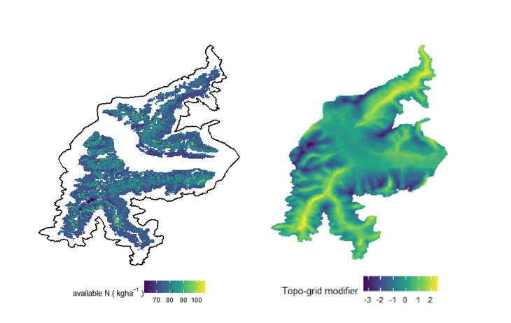
Figure S1. Additional figures showing spatially continuous parameters as input data in the model. Left: plant available nitrogen (kg ha^-1 year^-1) displayed only for the area covered by forest (see section on Biophysical parameters). Right: topex-to-distance map showing the topo-grid modifier used to scale wind effect across the study area by adding these values to estimated wind speeds (see section on Climate).

Table S1. Description of the different deadwood and soil carbon pool variables available from the Italian forest inventory (INFC) that we related to the spatially distributed parameters needed in iLand (e.g., swdC, youngRefractoryC). Number of plots indicates from how many INFC plots were the data retrieved and imputed to the forest categories of our study area. 

INFC			iLand
Code	Description	n. plots	Code	Description
Capm_ha	Standing dead trees (snags)	251	swdC	Carbon content in standing woody debris
Cce_ha	Stumps	251	youngRefractoryC	Carbon content in the pools for other wood (branches and coarse roots)
Cne_ha	Coarse woody debris (dbh > 9.5 cm)	251
Cnef_ha	Fine woody debris (dbh < 9.5 cm)	58	youngLabileC	Carbon content of litter pool
Clt_ha	Litter carbon pool	58
Cor_ha	Forest floor (organic  surface layer)	58	somC	Carbon content of soil organic matter - soil pool
Css_ha	Mineral surface horizon (soil depth <= 10 cm)	58
Csp_ha	Mineral horizon (soil depth 10-30 cm)	58

Table S2. Accuracy of the climate clustering. The numbers indicate the deviation of the clusters to the real data points (100m cells). For example, with N=800 clusters, 95 of the cells have a deviation in mean annual temperature from their original value ≤ 0.611. The final number of clusters was chosen to be 800 (*).

	ΔT (°C)		ΔPrecip (mm)		ΔRad (kWh/m²)
n. clusters	95% ≤	50% ≤	95% ≤	50% ≤	95% ≤	50% ≤
100	1.157	0.360	19.116	6.547	1.429	0.406
200	0.920	0.293	15.433	5.110	1.186	0.326
300	0.832	0.256	13.313	4.330	1.065	0.293
400	0.779	0.238	12.133	4.012	0.958	0.258
500	0.700	0.221	10.923	3.727	0.894	0.247
600	0.672	0.209	10.452	3.602	0.839	0.224
700	0.644	0.200	9.862	3.248	0.806	0.214
800*	0.611	0.188	9.424	3.145	0.761	0.205
900	0.588	0.181	9.153	2.978	0.735	0.191
1000	0.572	0.174	8.663	2.869	0.713	0.183
1200	0.536	0.164	8.207	2.707	0.650	0.171
1400	0.507	0.153	7.746	2.542	0.628	0.167
1600	0.480	0.143	7.423	2.438	0.600	0.154

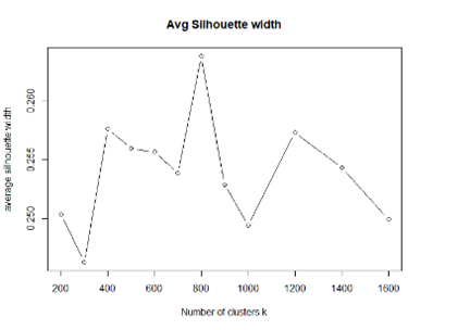
Figure S2. The average silhouette width for the number of climate clusters evaluated.

Table S3. Acronyms of the tree species used in iLand and their relative names.

iLand code	Tree species		iLand code	Tree species
abal	Abies alba		pimu	Pinus mugo
acca	Acer campestre		pini	Pinus nigra
acpl	Acer platanoides		pisy	Pinus sylvestris
acps	Acer pseudoplatanus		poni	Populus nigra
algl	Alnus glutinosa		potr	Populus tremula
alin	Alnus incana		psme	Pseudotsuga menziesii
alvi	Alnus viridis		qupe	Quercus petraea
bepe	Betula pendula		qupu	Quercus pubescens
cabe	Carpinus betulus		quro	Quercus robur
casa	Castanea sativa		rops	Robinia pseudoacacia
coav	Corillus avellana		saca	Salix caprea
fasy	Fagus sylvatica		soar	Sorbus aria
frex	Fraxinus excelsior		soau	Sorbus aucuparia
lade	Larix decidua		tico	Tilia cordata
piab	Picea abies		tipl	Tilia platyphyllos
pice	Pinus cembra		ulgl	Ulmus glabra

Table S4. Information on the management units (MU) covering the study area. MU indicate the code used in iLand to define unique management units linked to stand ids. The year indicates the latest renewal of the forest management plan for which most up-to-date information was available at the moment of data collection (2021). The period indicates the period of reference valid for the planning of future interventions.

MU	Name (German/Italian)	Ownership	Year	Period
1	Glurns / Glorenza	Public (Town)	2013	2014-2023
2	Schludern / Sluderno	Public (Town)	2011	2012-2021
3	Stilfs / Stelvio	Public (Hamlet)	2018	2019-2028
4	Laas / Lasa	Public (Hamlet)	2019	2020-2029
5	Tschengls / Cengles	Public (Hamlet)	2010	2011-2020
6	Matsch / Mazia	Public (Hamlet)	2015	2016-2025
7	Lichtenberg / Monte Chiaro	Public (Hamlet)	2011	2012-2021
8	Sulden / Solda	Public (Hamlet)	2012	2013-2022
9	Tartsch / Tarces	Public (Hamlet)	2018	2019-2028
10	Mals / Malles	Public (Hamlet)	2012	2013-2022
11	Prad / Prato	Public (Hamlet)	2010	2011-2020
12	Domane Sulden / Demanio Solda	Public (Province)	2015	2016-2025
13	Alliz / Alliz	Private (Collective)	2014	2015-2024
14	Tanas / Tanas	Private (Private owners)	2018	2019-2028

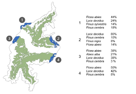
Figure S3. The forested areas outside the active simulation area, with their estimated species composition. These areas were considered to define the external seed belt that influences shading, external seed availability and the wind module. The rest of the stockable area, instead, bordered with natural barriers to seed dispersal, such as alpine rocks, ridge tops and urban settlements. Additional descriptions of the seed belt in iLand are available in the online documentation of the model (https://iland-model.org/external+seeds)

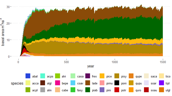
Figure S4. Development of forest succession averaged across the entire study area from bare ground over 1500 years in the absence of natural disturbances or management. For species names and codes see Table S3.

Disclaimer/Publisher’s Note:

The statements, opinions and data contained in all publications are solely those of the individual author(s) and contributor(s) and not of Forest Business Analytics and/or the editor(s). Forest Business Analytics and/or the editor(s) disclaim responsibility for any injury to people or property resulting from any ideas, methods, instructions or products referred to in the content.